1 System Requirements

You need Matlab installed and activated on your system to use Automagic. Automagic was developed and tested in Matlab R2015b and newer releases.

 

2 Installation

1. Go to the GITHUB repository https://github.com/amirrezaw/automagic

2. Download and unzip automagic-master to your favorite place on your hard drive.

 

3 How to use Automagic

 

3.1 Automagic directory hierarchy

Automagic assumes that single EEG recordings are stored within a folder of a subject. Each subject is stored in a project folder:

Project
|

Subject1

|

S1_EEGfile1

S1_EEGfile2

S1_EEGfile3

Subject2

|

S2_EEGfile1

S1_EEGfile2

…

 

3.2 Start Automagic

1. To run automagic, start Matlab and change your working directory to /automagic-master

2. Type RunAutomagic and the project gui (Figure 1) will appear*

*(Note that automagic will unzip certain files when started the first time, which can take some time)

 

Figure 1. Project GUI.

 

 

3.3 How to create a new project

 

1. Start Automagic (3.1)

2. Navigate to the drop-down list Select Project

3. Select Create New Project…

4. Name your project

5. Choose the folder where the raw data is

6. Optional. Choose the folder where you want to save your preprocessed data

7. Choose the EEG System that was used to record your data:

   1. You always have to provide the file extension that corresponds to your data file format.

   2. For Electrical geodesics (EGI HCGSN) recordings with 128 and 256 channels (or if the reference is included 129 and 257 respectively), everything is preset.

   3. If you are working with another EEG system click on Other...

8. Exclude channels that you do not want to include in your further processing by typing the channel indices (not the labels!) into Exclude

9. Channel location file:

   1. Unless your data contains an EEGLAB EEG structure with channel locations (EEG.chanlocs) included (or is an EGI file), you need to provide a file (supported by EEGLAB (pop_chanedit function)) in which channel locations are specified.

   2. The Channel location file must be the full address of the channel location file.

   3. The Channel location file type must specify the type of the file as required by pop_chanedit. eg. sfp

10. Indicate the sampling rate in Hz unless it is indicated in the EEG structure

 

By now you could simply press the create project button and you would have created a new project, ready to be preprocessed. However, depending on your data, it is you should consider to change to default configurations for the preprocessing methods that are implemented Automagic.

 

3.4 Setup the configurations

 

Click on Configurations (no worries, everything selected is save) to open the configurations GUI (see Figure 2)

Automagic offers several methods to detect bad channels that are later interpolated. Typically, either PREP or the clean_rawdata() pipelines work very well, so we recommend to choose either of them. We noticed that ASR in the clean_rawdata() not always yields replicable outcomes, but it might work for your data, so just test it! An additional method is implemented that searches for residual bad channels after having run the entire preprocessing pipeline. It catches the rare cases, when the other pipelines missed a channel with very high variance.

 

1. In the artifact removal panel you can select EOG-regression and either MARA or robustPCA.

   1. In the EOG - regression (Parra et al. 2005), EOG electrodes are used as a reference signal that is subtracted in proportion to their contribution to each EEG channel. Unless you are using EGI data, indicate the indices of the EOG channels, separated by white space.

   2. MARA performs and ICA and detects and rejects artifactual independent components (Winkler et al. 2011; Winkler et al. 2014). The ICA of MARA works best if the data is high pass filtered, so we recommend to filter the data with 1 Hz. Note that this filtering is only temporary.  

   3. The implemented algorithm (Inexact Augmented Lagrange Multiplier Method for PCA (Lin et al. 2010) estimates a low-dimensional subspace of the observed data, reflecting the signal that is cleaned from sparse corruptions. This method is generally faster, but has removed less artifacts than MARA as we have observed in validations. Unless you deliberately tuning the robust PCA, the default parameters work well for many situations.

2. Filtering

   1. Line Power: Indicate if you would like to apply a notch filter to your data. Note that using PREP already takes care of line noise using CleanLine (Mullen 2012). Indicate the line power where your EEG was recorded

   2. High Pass Filter: Check the box if you would like to apply a high pass filter and indicate the cutoff frequency. The filer order will be estimated according to eeg_filtnew() of EEGLAB by default.

   3. Low Pass Filter: Check the box if you would like to apply a low pass filter and indicate the cutoff frequency. The filer order will be estimated according to eeg_filtnew() of EEGLAB by default.

3. Quality Rating

   1. The Overall Thresholds is a list of absolute voltage magnitudes in mV at which the ratio of data points (i.e. channels x timepoints) that have a higher absolute voltage magnitude than that threshold is calculated.

   2. The Time Thresholds is a list of values of standard deviations of voltage magnitudes in mV whitin time points (across channels) at which the ratio of timepoints that have a higher standard deviation than that threshold is calculated.

   3. The Channels Thresholds is a list of values of standard deviations of voltage magnitudes in mV whitin channels (across time) at which the ratio of channels that have a higher standard deviation than that threshold is calculated.

4. Interpolation

   1. The interpolation method can be selected here. Refer to the help of eeg_interp() for details on the methods.

5. Downsampling Rate

   1. The downsampling only affects the visual representation of your data. A higher downsampling rate will shorten loading times and reduce memory need. In general, a downsampling rate of 2 is a good choice.

6. Confirm your configurations by clicking OK.

7. In the Project GUI create your project by clicking the button Create Project. Once the configurations are defined and a study is created, all the configurations are fixed and cannot be changed any more to assure that all datasets of a project are identically processed. In contrast to having the configurations fixed, the input files are not, that is, it is always possible to add (or to delete) datasets to a data folder and Automagic detects these changes whenever the application is restarted. This guarantees that all EEG files are preprocessed in a standardized way.  

Figure 2. Configurations

 

3.5 Run the preprocessing

1. ...by clicking Run in the Preprocessing panel

 

3.6 Bad Channel Interpolation

After preprocessing has finished you will be notified with a pop-up message. Now you can either review the data and inspect which channels have been detected as bad channels and how the artifact removal and filtering has changed your raw data using the Review Data button or you can interpolate the bad channels straight away by clicking Interpolate.

3.7 Quality Assessment

The quality assessment GUI (see Figure 3) gives an overview of each dataset that has been preprocessed.

1. The data is plotted as a heatmap (MATLABs imagesc plot) with time points on the x axis and channels on the y axis. The color of each data point reflects the voltage magnitude. As artifacts are typically of higher amplitude than the EEG signal of interest, red and blue data points that stand out of the mostly green data points typically indicate some sort of noise.

   1. The color scaling (min und max values) can be changed with the scrollbar in the lower right corner. These values might differ between recording systems.

   2. The Average Reference button changes the data rendered to average referenced data.

   3. Auto Bad channels shows the automatically detected bad channels in blue lines (this only applies to data before interpolation)

   4. View Raw File shows a 1 Hz high pass filtered plot of your data, which can be used to compare the noise before and after preprocessing.

2. The right panel shows an automated rating of the quality of the current data set that is based on a series of Quality scores (explained later)

   1. The user can override these quality scores (but we do not recommend to do so) and can manually select channels that have not been identified as bad by either of the methods. These channels can be interpolated.

3. In the top panel, you can make a selection of, for example only the datasets that are rated as Good. This allows to quickly scroll through the datasets by clicking on Previous or Next.

4. Clicking the EEGLAB plot opens a new figure that shows the current data set in the EEGLAB channel plot.

5. Clicking the Quality Rating button additionally opens the quality rating GUI.

 

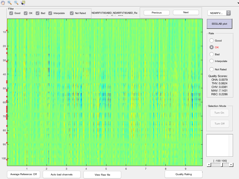
Figure 3. Quality Assessment

 

3.8 Quality Rating

The quality rating GUI allows to categorize your data into “Good”, “Ok” and “Bad” datasets. This should serve as an objective way of including / excluding datasets into further analyses. Currently four quality measures are computed which all reflect ratios (range from 0 to 1):

1. The overall high amplitude (OHA) measure reflects the ratio of data points (i.e. channels x timepoints) that have a higher absolute voltage magnitude of x mV, where x reflects a vector of voltage magnitude thresholds (set in the configurations).

2. The timepoints of high variance (THV) measure reflects the ratio of  time points, where the standard deviation of the voltage measures across all channels exceeds x mV, where x reflects a vector of standard deviation thresholds (set in the configurations).

3. The channels of high variance (CHV) measure reflects the ratio of channels for which the standard deviation of the voltage measures across all time points exceeds x mV, , where x reflects a vector of standard deviation thresholds (set in the configurations).

4. The ratio of bad channels (RBS) reflects the ratio of interpolated bad channels.

 

Using a selection of the quality measures (OHA, THV, CHV,  RBC) and specified thresholds, the you can classify the datasets of a project into three categories “Good”, “Ok”, “Bad”, by applying cutoffs for each criterion (see Figure 4). All the values for thresholds and category cutoffs can be modified and therefore the user can compile samples in accordance to own purposes. The thresholds can be changed in the respective dropdown menu on the right side. This influences the sensitivity of a quality measure. The cutoff for a category (“Good”,”Ok”,”Bad”) can be modified using the respective sliders. To make the effect of the modifications visible, the resulting ratings for the currently displayed dataset (in the quality assessment GUI) is adapted. In addition, the frequencies of each categories is plotted in the barplot, so you can also base your categorization on the resulting sample sizes. To restrict yourself in compiling categories and running analyses until effects become true (i.e. P-hacking), you can commit a selected categorical assignment by pressing “commit rating”, which appends the letters “g” for “Good”, “o” for “Ok”, and “b” for “Bad” to the file name of the preprocessed EEG dataset. There is a Reset rating button but as a sincere researcher you should not press it.

 

Figure 4. Quality Rating GUI

 

4 More Information

 

4.1 While running Automagic...

 

You can not close the GUI during the preprocessing. If you wish to stop the preprocessing at any time, hit CTRL-C. In this case, or if by any other reason the preprocessing is stopped before being completely finished, all preprocessed files to that moment will be saved, and you can resume the preprocessing only for the files which are not preprocessed yet. After having used CTRL-C, please load your project from the GUI, by reselecting it from the list of existing projects. This will update the GUI with the new preprocessed files. Note: Since synchronisation is rather basic, people should never work on the same project simultaneously from different devices.

4.2 Loading an Existing Project

If you already had created a project and for some reasons re-installed your matlab or Automagic, you can load that project and keep all the information. There are two options to load an existing project. The first option can only be used to open projects that have been created on your system or that have been loaded before:

1. Navigate to the drop-down list labelled Select Project.

2. Select the project you want to load.

The second option can be used to load any Automagic project:

1. Navigate to the drop-down list labelled Select Project.

2. Select Load an existing project...

3. A browser window will open. Navigate to the existing project...s project folder.

4. Select and open the file named project_state.mat

5. Indicate the folder with the data

 

4.3 Merging Projects

To merge any number of existing projects without losing the individual projects, please follow these steps:

1. Create a new data folder using Finder (Mac), Explorer (Windows) or your Linux equivalent.

2. Create a new project folder using Finder (Mac), Explorer (Windows) or your Linux equivalent.

3. For all the projects that you want to merge: Copy the contents from the data and project folders to the new data and project folders.

4. Important: Each of your existing project folders contains a file named project_state.mat. Do not copy these files to your new project folder.

5. In Automagic: Create a new project using the newly created data and project folders.

 

4.4 Adding Data to an Existing Project

If you would like to add some new data:

1. Add subject folders to your data folder using Finder (Mac), Explorer (Windows) or your Linux equivalent.

2. Refresh the Automagic GUI using one of these options:

3. Start or restart Automagic.

4. Navigate to the drop-down list labelled Select Project and load (or reload) the project containing new data by clicking on its name.

5. The number of subjects and files in both the project panel and the pre-processing panel should now be updated.

4.4 Deleting Data from an Existing Project

1. Delete subject folders from your data folder using Finder (Mac), Explorer (Windows) or your Linux equivalent.

2. Refresh the Automagic GUI:

3. Navigate to the drop-down list labelled Select Project and load (or reload) the project containing new data by clicking on its name.

4. The number of subjects and files in both the project panel and the pre-processing panel should now be updated.

 

4.6 Deleting a Project

1. Click on Delete Project in the lower right corner of the project panel. A dialog box will appear. Take responsibility by clicking on Delete.

2. Note: This will only delete the file named project_state.mat in the project folder and remove the project from the Automagic GUI.

3. Please use Finder (Mac), Explorer (Windows) or your Linux equivalent to delete your project data and/or project folder.

 

4.5 References

References of used functions in Automagic:

Bigdely-Shamlo, N., Mullen, T., Kothe, C., Su, K. M., & Robbins, K. A. (2015). The PREP pipeline: standardized preprocessing for large-scale EEG analysis. Frontiers in neuroinformatics, 9, 16.

Lin, Z., Chen, M., & Ma, Y. (2010). The augmented lagrange multiplier method for exact recovery of corrupted low-rank matrices. arXiv preprint arXiv:1009.5055.

Mullen, T., Kothe, C., Chi, Y. M., Ojeda, A., Kerth, T., Makeig, S., ... & Jung, T. P. (2013, July). Real-time modeling and 3D visualization of source dynamics and connectivity using wearable EEG. In Engineering in Medicine and Biology Society (EMBC), 2013 35th Annual International Conference of the IEEE (pp. 2184-2187). IEEE.

Winkler, I., Brandl, S., Horn, F., Waldburger, E., Allefeld, C., & Tangermann, M. (2014). Robust artifactual independent component classification for BCI practitioners. Journal of neural engineering, 11(3), 035013.

Winkler, I., Haufe, S., & Tangermann, M. (2011). Automatic classification of artifactual ICA-components for artifact removal in EEG signals. Behavioral and Brain Functions, 7(1), 30.